1.2. The First Derivative#
Note
Important things to retain from this block:
Understand what the derivative represents
Recognize that the derivative can be approximated in different ways
In your calculus classes, you might remember working with the analytical definition of a derivative, such as \(\frac{df}{dx}\). This involved finding the limit as the distance between two points becomes infinitesimally small.
The derivative of a function \(f(x)\) evaluated at the point \(x_0\) is
\(x - x_0\) cannot tend to 0! Thus:
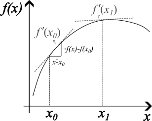
Fig. 1.2 derivatives of a function \(f(x)\) at a specific points \(x_0\) and \(x_1\)#
What does the derivative represents? A rate of change! In this case, how fast \(f(x)\) changes with respect to \(x\) (or in the direction of \(x\)). The derivative can also be with respect to time or another independent variable (e.g., \(y,z,t,etc\)). Look at the figure above. The first derivative evaluated at \(x_0\) is illustrated as a simple slope, as is the first derivative evaluated at \(x_1\) . You can also see that the rate of change at \(x_0\) is larger than at \(x_1\).
Numerical Freedom to compute derivatives#
In the Figure above, the derivative approximation was illustrated arbitarly using two points: the one at which the derivate was evaluated and another point in front of it. However, there are more possibilities. Instead of using absolute points at \(x_{-1,0,1}\) a more general notation is used: \(x_{i-1,i,i+1}\). The simplest ways to approximate the derivative evaluated point \(x_i\) is to use two points:
Note that the finite difference formula requires distances \(x_{i+1}-x_i\) and \(x_i-x_{i+1}\). This will be introduce in the next chapter ‘FDM intro’ and will become more evident in the ‘Taylor Series Expansion chapter’.
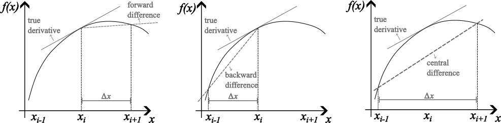
Fig. 1.3 graphs illustrating three different ways to approximate derivatives.#