1.3. Finite Difference Method

The Finite Difference Method (FDM) is an indispensable numerical approach, which plays a fundamental role in solving differential equations that govern physical phenomena. In this method, the derivatives in the differential equation are approximated using numerical differences, just like the forward, backward and central differences treated in the previous chapters.

Consider the following equation that describes ice growth of an ice layer assuming that the air and water temperatures are constant:

\[ \rho_{ice}\frac{dh_{ice}}{dt}=-k_{ice}\frac{T_{water}-T_{air}}{h_{ice}} \]

where \(h_{ice}\) is the ice thickness, \(\rho_{ice}\) ice density and \(k_{ice}\) refers to the heat transfer capabilities of the ice.

The growth rate (derivative) if the ice thickness can be approximated with one of the numerical derivatives and the resulting equation can be solved for the ice thickness in the next time step. In essence, the finite difference method transforms a differential equation into an algebraic form (discretization).

Still a definition of the solution domain is needed. For this example, an inital and an end time \([a,b]\), where \(a\) and \(b\) are called end points. The domain is represented as grid points and therefore in a number of subintervals \(N\). The length of the subinterval is \(h=(b-a)/N\).

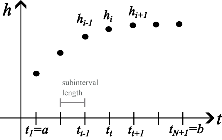
Fig. 1.4 Discretized differential equation ``

The figure above shows the grid of which the following property holds:

\[ a=t_1 < t_2 < ..<t_{N}< t_{N+1}= b \]

The Points \(t_i\) on the grid are called nodes. Just note that your indexing is a choice. For example \(i\) can be for \(i = (1,2,...,N, N+1)\) as shown in the figure above. The indexing can also start at 0 where \(i = (0,1,...,N-1, N)\).

Lets simplify the above ice equation and put it in a standard ODE form:

\[ \frac{dh}{dt}= f \]

We can rewrite this equation in a discretize form:

\[ h'_i = f_i \]

Note that \(h'_i\) is the first derivative at node \(i\) and at that node is equal to function \(f_i\). Using FDM we numerically compute the solution \(h_i\) at each node \(t_i\) The connection between the derivative \(h'_i\) and \(t_i\) can be made by using Taylor Series Expansions.