1.8. Boundary-value Problems: second-order ODE

To solve a first order ODE, one constraint is needed (initial value problem, IVP). In the case of a second order ODE, two constraints are needed. If the constraints are defined at different locations of the domain, then you will be dealing with a Boundary-value problem (BVP). Mostly when we use time derivatives we have an IVP and when we have a derivative in space we have to deal with spacial constraints and therefore BVP’s. See the following examples:

\[ \frac{dp}{dt} = -p^{3/2} + 5*p_{cst}(1-e^{-t}) \text{ first order ODE -> IVP with 1 constraints } p[0] = 1000 \]

\[ \frac{d^2y}{dt^2} = \frac{dy}{dt} -y + \cos t =0 \text{ second order ODE -> IVP with 2 constraints } y[0] = 2 \text{ and } \left. \frac{dy}{dt} \right|_{t=0} = 5 \]

\[ \frac{d^2T}{dx^2}-\alpha_1(T-T_s) =0 \text{ second order ODE -> BVP with 2 constraints } T[0] = 10 \text{ and }T[-1] = 20 \]

Even for higher ODE orders, the number of constrains required corresponds to the order of the ODE. It is clear that a second order ODE can either be an IVP or a BVP. The former case is common when describing time derivatives and the latter case is common when describing space derivatives. From now on, we focus on BVP.

Boundary Conditions

A second order ODE BVP of the type:

\[ \frac{d^2y}{dx^2} = g(x,y,\frac{dy}{dx}) \]

with a domain solution \(a<=x<=b\) and boundary conditions (or constraints) defined at \(a\) and \(b\) typically has two types of boundary conditions:

• Dirichlet boundary conditions

\[ y(x=a) = Y_a \text{ and } y(x=b) = Y_b \]

• Neumann boundary conditions

\[ \left. \frac{dy}{dx} \right|_{x=a} = D_a \text{ and } \left. \frac{dy}{dx} \right|_{x=b} = D_b \]

Of course, a combination of BC can also exist.

Consider the following equation that describes the deformation \(y\) of a beam with length \(L\) clamped at \(x=0\) and \(x=L\):

\[ \frac{d^4y}{dx^4}=\alpha \text{ load}(x) \]

where \(\alpha\) represents the beams material characteristics.

As it is and ODE of fourth order, it needs 4 BCs. The nature of the problem states that the deformation and the slope of the deformation at the ends is 0, thus, two Dirichlet and two Neumann BCs:

\[ y(0)=0; \left. \frac{dy}{dx} \right|_{x=0}=0; \hspace{5mm} y(L)=0; \left. \frac{dy}{dx} \right|_{x=L}=0; \]

Fig. 1.15 Illustrating the boundary conditions of a fourth order ODE that describes the deformation of a beam

Solving a BVP using Finite Differences

Just like in the initial value problem section, here the derivatives are approximated numerically following a desired method and order of accuracy. Now the domain going from \(a\) to \(b\) is discretized using a determined number of grid points \(n\) and, thus, a number of sub-intervals \(N\). There is always one more point than sub-intervals, \(n=N+1\). This is the grid (see Figure below) and, if the spacing is regular, then the length of the sub-interval is \(\Delta x = (b-a)/N\).

Fig. 1.16 Illustration of the grid, highlighting the two external boundary nodes with known temperatures (\(T\)) and the internal nodes where the temperature values must be estimated.

The Boundary Conditions are defined at the end points and the discretization is applied at almost every point. This depends on the numerical approximation. The following steps are followed to solve a BVP:

1. Discretization of the differential equation with a numerical approximation of choice

2. Parameter definition

3. Grid creation

4. Define Boundary conditions

5. Building a system of equations according to the discretization: \(Ay=b\)

6. Solving the system

Lets visualize these steps above with an exercise:

Let’s consider the following problem 2nd order differential equation BVP:

\[ \frac{d^2T}{dx^2} - \alpha(T-Ts)= 0, \hspace{5mm} x \in(0,0.1) \]

\[ T(0)= 473 [K], \hspace{3mm} T(0.1)= 293 [K] \]

The parameter \(\alpha=166\) and your starting temperature \(Ts= 293 [K]\)

Use the Finite Central Difference method to approximate the above differential equation at 5 equally spaced intervals.

\[ \text{Central Difference: } f''= \frac{f(x_i-\Delta x)-2f(x_i)+f(x_i+\Delta x)}{\Delta x^2}+ \mathcal{O}(\Delta x)^2. \]

Click here for the derivation of the 2nd order central finite difference method

Solution:

Remember the trick: 2nd order derivative and 2nd error order (2+2=4), so expand the Taylor series until the 4th order

\[ f(x_{i+1}) = f(x_i) + \Delta x f'(x_i) + \frac{\Delta x^2}{2} f''{x_i} + \frac{\Delta x^3}{6} f'''_{x_i} + \mathcal{O}(\Delta x^4) \]

\[ f(x_{i-1}) = f(x_i) - \Delta x f'(x_i) + \frac{\Delta x^2}{2} f''{x_i} - \frac{\Delta x^3}{6} f'''_{x_i} + \mathcal{O}(\Delta x^4) \]

Now, summing the two expansions (for \( x_{i+1}\) and \( x_{i-1} \)):

\[ f(x_{i+1}) + f(x_{i-1}) = 2y(x_i) + \frac{\Delta x^2}{2} f''{x_i} + \mathcal{O}(\Delta x^4) \]

Rearranging to isolate the second derivative and divide by \(\Delta x^2\):

\[ f''= \frac{f(x_i-\Delta x)-2f(x_i)+f(x_i+\Delta x)}{\Delta x^2}+ \mathcal{O}(\Delta x). \]

1. First discretize the differential equation

We use the Central Difference method to discretize our above differential equation

\[ \frac{1}{\Delta x^2}(T_{i-1}-2T_{i}+T_{i+1}) - \alpha (T_i - Ts) =0 \]

2. Define parameters

Our parameters are \(\alpha\) and Ts

3. Define your grid

We want 5 equally spaced intervals. \(\Delta x = (0.1-0)/5= 0.02\) and \(\Delta x^2= 0.0004\)

Define the grid: \(x_0= 0, x_1= 0.02, x_2= 0.04, x_3= 0.06,x_4= 0.08, x_5= 0.1\)

4. Define boundary conditions

Our external nodes \(x_0\) and at \(x_5\) are our dirichlet boundary conditions, which are our known solutions at:

\[ T_0= 473 [K], \hspace{3mm} T_5= 293 [K] \]

5. Building a System of Equations:\( \mathbf{A} \mathbf{T} = \mathbf{y} \)

We will use the central difference method to approximate the derivative at the internal nodes.

For \(i = 1\): The finite difference approximation for the first internal node is:

\[ \frac{1}{\Delta x^2}(T_0 - 2T_1 + T_2) - \alpha T_1 + \alpha T_s = 0 \]

Next, we multiply by \(\Delta x^2\) and substitute the boundary condition for \(T_0\). Notice that the only unknown solutions are \(T_1\) and \(T_2\) Rearranging the terms gives:

\[ -(2 + \alpha \Delta x^2) T_1 + T_2 = -\alpha T_s \Delta x^2 - T_0 \]

For \(i = 2\): The finite difference approximation for the second internal node is:

\[ \frac{1}{\Delta x^2}(T_1 - 2T_2 + T_3) - \alpha T_2 + \alpha T_s = 0 \]

Rearranging the terms:

\[ T_1 - (2 + \alpha \Delta x^2) T_2 + T_3 = -\alpha T_s \Delta x^2 \]

For \(i = 3\): The finite difference approximation for the third internal node is:

\[ \frac{1}{\Delta x^2}(T_2 - 2T_3 + T_4) - \alpha T_3 + \alpha T_s = 0 \]

Rearranging the terms:

\[ T_2 - (2 + \alpha \Delta x^2) T_3 + T_4 = -\alpha T_s \Delta x^2 \]

For \(i = 4\)

\[ \frac{1}{\Delta x^2}(T_3-2T_4+T_5) - \alpha T_4 + \alpha Ts =0 \]

Notice that now we can plug in our other bc \(T_5\) and rearrange the terms:

\[ (T_3 - (2 + \alpha \Delta x^2) T_4 ) = -\alpha Ts \Delta x^2 -T_5 \]

We can now move the equations in the Ax=y form:

\[\begin{split} \begin{bmatrix} -(2 + \alpha \Delta x^2) & 1 & 0 & 0 \\ 1 & -(2 + \alpha \Delta x^2) & 1 & 0 \\ 0 & 1 & -(2 + \alpha \Delta x^2) & 1 \\ 0 & 0 & 1 & -(2 + \alpha \Delta x^2) \end{bmatrix} \begin{bmatrix} T_1 \\ T_2 \\ T_3 \\ T_4 \end{bmatrix} = \begin{bmatrix} -\alpha Ts \Delta x^2 -T_0\\ -\alpha Ts \Delta x^2 \\ -\alpha Ts \Delta x^2\\ -\alpha Ts \Delta x^2 -T_5 \end{bmatrix} \end{split}\]

Below you can see how we can put the above steps into code:

We can now estimate the temperature T at each node.

import numpy as np 
import matplotlib.pyplot as plt


dx=0.02
Ts = 293
alpha = 166
matrix_element = -(2+dx**2*alpha)
b_element = -dx**2*alpha*Ts

# grid creation
x = np.arange(0,0.1+dx,dx)
T = np.zeros(x.shape)

# boundary conditions
T[0] = 473
T[-1] = 293

# Building matrix A
A = np.zeros((len(x)-2,len(x)-2))
np.fill_diagonal(A, matrix_element)
A[np.arange(3), np.arange(1, 4)] = 1  # Upper diagonal
A[np.arange(1, 4), np.arange(3)] = 1  # Lower diagonal
b = np.array([ b_element - T[0] , b_element, b_element,  b_element - T[-1]])

# Solving the system
A_inv = np.linalg.inv(A)
T[1:-1] = A_inv @ b


plt.plot(x,T,'*',label='Estimated solution')
plt.xlabel('x')
plt.ylabel('T')
plt.title('Estimated solution using Central Difference method')
plt.legend()
plt.show()

print(f'The estimated temperature at the nodes are: {[f"{temp:.2f}" for temp in T]} [K]')

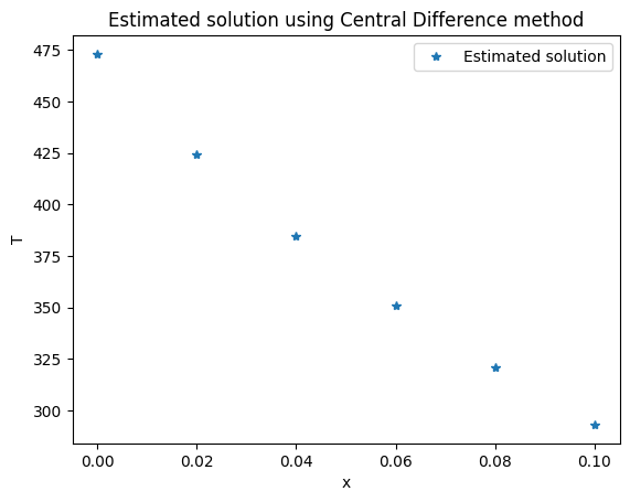
The estimated temperature at the nodes are: ['473.00', '424.46', '384.64', '350.91', '321.02', '293.00'] [K]

Summary of Finite Difference methods

First order derivative Finite Difference Methods

\[ \text{Backward Difference: } f'= \frac{f(x_i)-f(x_{-1})}{\Delta x} + \mathcal{O}(\Delta x) \]

\[ \text{Forward Difference: } f'= \frac{f(x_{i+1})-f(x_1)}{\Delta x}+ \mathcal{O}(\Delta x) \]

\[ \text{Central Difference: } f'= \frac{f(x_{i+1})-f(x_{i-1})}{2\Delta x}+ \mathcal{O}(\Delta x)^2 \]

Second order derivative Finite Difference Methods

\[ \text{Backward Difference: }f''(x_i)=\frac{f(x_i)-2f(x_{i-1})+ f(x_{i-2})}{\Delta x^2}+ \mathcal{O}(\Delta x). \]

\[ \text{Forward Difference: }f''(x_i)=\frac{f(x_{i+2})-2f(x_{i+1})+f(x_i)}{\Delta x^2}+ \mathcal{O}(\Delta x). \]

\[ \text{Central Difference: } f''= \frac{f(x_{i-1})-2f(x_i)+f(x_{i+1})}{\Delta x^2}+ \mathcal{O}(\Delta x)^2. \]

For if you want a bit more practice.

Exercise

Here is a second order derivative BCP:

\[ f''= x^2, \hspace{5mm} x \in(0,1) \]

\[ f(0)=1, f(1)=1 \]

Divide the domain [0,1] into 5 equal intervals and apply the Central Finite Difference to estimate \(f''\) at each grid node.

Solution

Discretize differential equation:

\[ f''_i \approx \frac{1}{\Delta x^2}(f_{i-1}-2f_i+f_{1+1}) \]

Define the grid:

\(\Delta x\) = (1-0)/5 = 0.2 Hence \(\frac{1}{\Delta x^2} = \frac{1}{0.2^2}= 25\)

\[ x_0 = 0, x_1 = 0.2, x_2= 0.4, x_3= 0.6, x_4= 0.8, x_5= 1 \]

Define BC:

\[ f_0= 1, \hspace{5mm} f_5= 1 \]

Set up a system of equations for internal nodes i= 1,…,4 :

\[ 25(f_0-2f_1+f_2)= 0.2^2 \]

\[ 25(f_1-2f_2+f_3)= 0.4^2 \]

\[ 25(f_2-2f_3+f_4)= 0.6^2 \]

\[ 25(f_3-2f_4+f_5)= 0.8^2 \]

Plugging in the bc \(f_0=1\) and \(f_5=1\) and moving the to the right-hand side:

\[ 25(-2f_1+f_2)= 0.2^2 - 25 \]

\[ 25(f_1-2f_2+f_3)= 0.4^2 \]

\[ 25(f_2-2f_3+f_4)= 0.6^2 \]

\[ 25(f_3-2f_4)= 0.8^2 - 25 \]

we can bring this to a system of linear equations of the form:

\[ \frac{1}{\Delta x^2}A\mathbf{f}=\mathbf{y} \]

\[\begin{split} 25\begin{bmatrix} -2 & 1 & 0 & 0 \\ 1 & -2 & 1 & 0 \\ 0 & 1 & -2 & 1 \\ 0 & 0 & 1 & -2 \end{bmatrix} \begin{bmatrix} f_1 \\ f_2 \\ f_3 \\ f_4 \end{bmatrix} = \begin{bmatrix} 0.2^2 - 25\\ 0.4^2 \\ 0.6^2\\ 0.8^2 - 25 \end{bmatrix} \end{split}\]