1.5. Numerical Integration#
NOTE
Note
Important things to retain from this block:
Know how to apply different discrete integration techniques
Have an idea on how the truncation errors change from technique to technique
Motivation#
Numerical integration is used often in diverse fields of engineering. For example to develop advanced numerical model techniques or to analyze field or laboratory data where a desired physical quantity is an integral of other measured quantitites. So, the analytic integral is not always known and has to be computed (approximated) numerically. For example, the variance density spectrum (in ocean waves) is a discrete signal obtained from the water level variations and its integral is a quantity that characterizes the wave field.
Discrete Integration#
In a 1 dimensional situation, the integral:
is defined between points and represents the area under the curve \(f\) limited by \([a,b]\). A visual way to approximate that area would be to use a squared page and count the number of squares that fall under that curve. In the example figure, you can count 11 squares.
The numerical integration is an approximation to that area done in a strict way. There are several paths to follow using polynomial representation. These widely used formulas are known as Newton-Cotes formulas.
First, we split the interval of integration (a,b) on several partial intervals.
Then, we replace \(f(x)\) by the interpolation polynomial in each interval and calculate the integral over it.
Finally, sum all the areas to find (approximate) the integral.
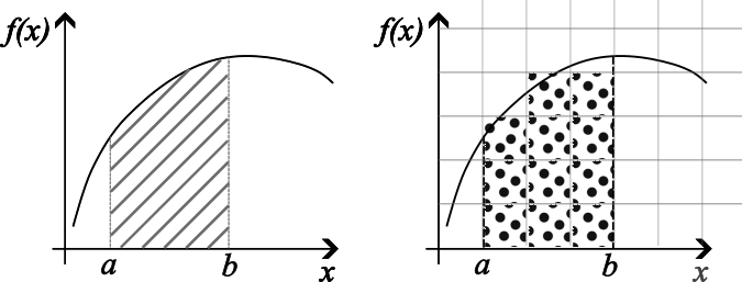
Fig. 1.5 two integral illustration showing the area under the curve for interval [a,b]#
Left Riemann Integration#
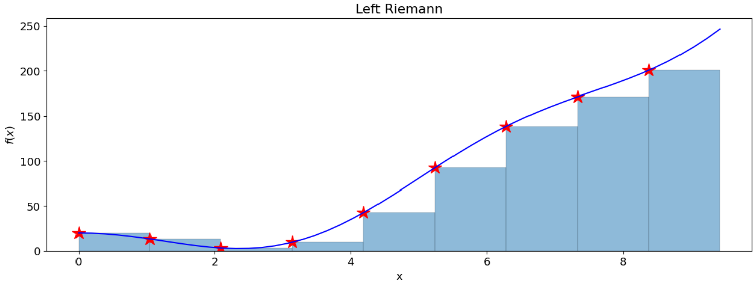
Fig. 1.6 Illustrating the left Riemann Sum over interval [a,b]#
Using the lowest polynomial order leads to the Riemann integral also known as the rectangle rule. Basically, the function is divided in segments with a known \(\Delta x\) and the area of each segment is represented by a rectangle. Its height, related to the discretized points of the function, can be defined by the left or by the right.
Therefore, we get the left Riemann integration formula given by:
where \(n\) is the number of segments.
Right Riemann Integration#
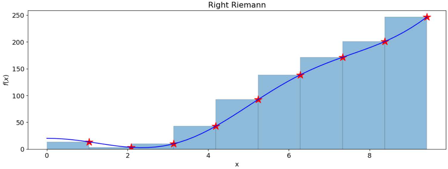
Fig. 1.7 Illustrating the right Riemann Sum over interval [a,b]#
In an analogous way, the formula for the right Riemann integration is:
Note the difference respect to the left Riemann integration, specially the starting and end points.
Midpoint Rule#
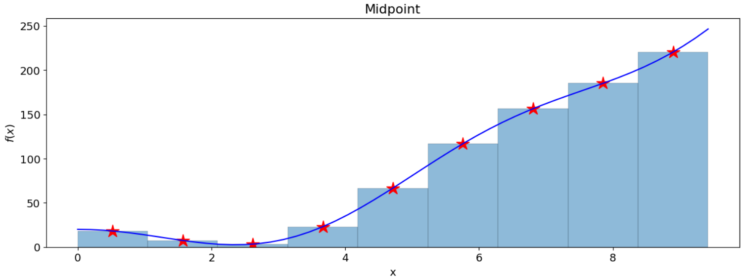
Fig. 1.8 Illustrating the right Midpoint Rule over interval [a,b]#
The midpoint rule defines the height of the rectangle at the midpoint between the two end points of each interval:
Trapezoidal Rule#
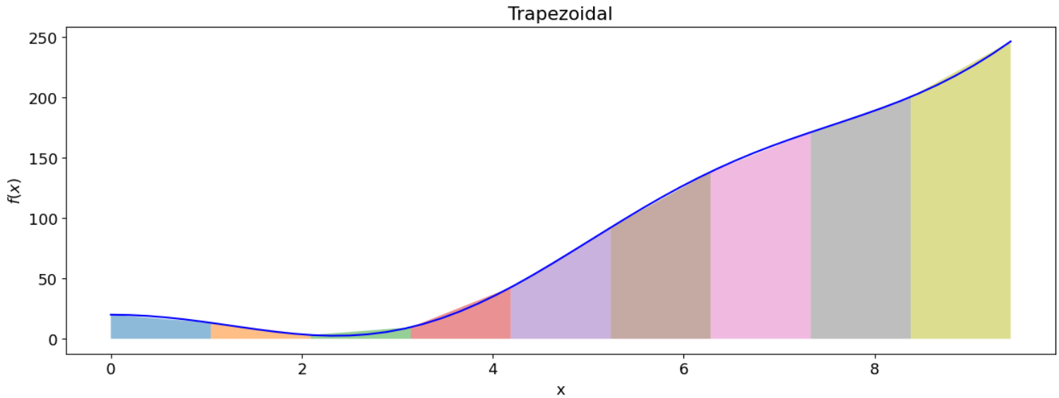
Fig. 1.9 Illustrating the Trapezoidal Rule over interval [a,b]#
The trapezoidal rule uses a polynomial of the first order. As a result the area to be computed is a trapezoid (the top of the rectangle has a slope now) where the bases are the values assumed by the function in the end points of each of the partial intervals, and its height is just the difference between two consecutive points. Mathematically it reduces to the average of two rectangles:
Simpson’s Rule#
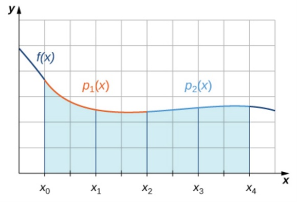
Fig. 1.10 Illustrating the Simpson Rule over interval [a,b]#
Simpson’s rule uses a second order polynomial. It computes the integral of the function \(f(x)\) by fitting parabolas needing three consecutive function points and adding the areas under them (see \(p_1(x)\) and \(p_2(x)\) in the figure). In formula form:
Note that the interval length is multiplied with two, since three points are needed.
Estimate the integral \(\int_{0.5}^1 x^4\) with a total number of steps n=2:
Left Riemann Sum
Midpoint rule
Trapezoidal
and then compute the real error \(\epsilon= | f(x)- \hat{f(x)|}\), where f(x) is the exact integral and \(\hat{f(x)}\) the approximated integral
Tip
Tip: feel free to use the code cell below as a calculator.
Solution
find \(\Delta x\),
Left Riemann Sum:
Midpoint Rule:
Trapezoidal Rule:
Exact
Error
error Left Riemann = \(| 0.19375 - 0.0947265625|\) = \(0.0990234375\)
error Midpoint Rule = \(| 0.19375 - 0.1846923828125|\) = \(0.009057617187500006\)
error Trapezoidal Rule = \(| 0.19375 - 0.2119140625|\) = \(0.018164062499999994\)
#feel free to use this as your calculator for the exercise above

def f(x):
    return x**4

f_left_riemann=
f_Midpoint=
f_trapezoidal=
f_exact=

print(f"f_left_riemann = {f_left_riemann}")
print(f"f_Midpoint = {f_Midpoint}")
print(f"f_trapezoidal = {f_trapezoidal}")
print(f"f_exact = {f_exact}")
print(f"Error left Riemann = {abs(f_exact-f_left_riemann)}")
print(f"Error Midpoint = {abs(f_exact-f_Midpoint)}")
print(f"Error trapezoidal = {abs(f_exact-f_trapezoidal)}")
Truncation Errors#
The truncation error for each method is the difference between the exact integral and the approximated integral. In the case of the left Riemann method:
Now, we can use the Taylor Series Expansion of \(f(x)\) instead of \(f(x)\) itself and solve that integral. If you are curious about the mathematical steps, further below you can find the detailed derivation. For the moment, let’s see the absolute errors for the different techniques.
Analysis#
As we can see, for the left and right Riemann integration techniques we find errors \(\sim \dfrac{1}{n}\), while for the midpoint and trapezoidal rules, we find them \(\sim\dfrac{1}{n^2}\), and with Simpson’s rule \(\sim\dfrac{1}{n^4}\).
Truncation Error Derivation for Left Riemann integration#
Note
You don’t need to know the derivation for the exam.
Derivation
Start by using a Taylor series expansion:
Substitute this Taylor expansion (2) in the term \(\int_a^b f(x)dx\) in equation (1):
Rewrite this as the sum of the integrals over the sub-intervals \([x_i,x_{i+1}]\):
Using integration by substitution, \(u= x-x_i\), therefore \(\frac{du}{dx}=1\) meaning du=dx
Plug equation (8) in equation (1):
The term \(\Delta xf(x_i)\) falls away:
\(\Delta x = \frac{b-a}{n}\) this gives:
The resulting left Riemann error is proportional to the average of the derivatives, the length of the domain (b-a) and the step size (\(\Delta x\)). This result tells us that for steeper functions the error will be higher than for milder ones. For example, a function of a straight horizontal line with average derivatives equal to 0 would have an error equal to 0! Also, the error will be larger if the domain is larger, which is kind of obvious. As those first two terms (average derivative and domain length) are inherent to the problem requirements, we say that the error is of the order \(\Delta x\).
Estimate the integral \(\int_{1}^{3} \frac{5}{x^4} dx\) with a step-size \(\Delta x= 0.5\)
Right Riemann Sum
Simpson Rule
Tip
Tip: feel free to use the code cell below as a calculator.
Solution
Find \(n\)
Right Riemann Sum
Simpsons Rule
Exact
error
#feel free to use this as your calculator for the exercise above
def f(x):
    return 5/(x**4)

f_right_riemann =
f_simps =
f_exact =

print(f"f_right_riemann = {f_right_riemann}")
print(f"f_simps = {f_simps}")
print(f"f_exact = {f_exact}")
print(f"Error right Riemann = {abs(f_exact-f_right_riemann)}")
print(f"Error Simpsons = {abs(f_exact-f_simps)}")